ROM vs dense FE sweep
This page compares two surrogates built from the same converged adaptive graph against a dense FE sweep on the one-parameter diffusion benchmark.
The model
The same 2D scalar diffusion problem as the one-parameter sweep:
-\nabla \cdot \bigl(c(\mu)\,\nabla u\bigr) \;=\; \lambda\,u \quad \text{in } \Omega = [0,1]^2, \qquad u = 0 \text{ on } \partial\Omega.
Two surrogates from one graph
Both surrogates consume the converged adaptive graph and make predictions at arbitrary \mu without additional FE solves. They differ in how they use the stored data:
Galerkin ROM (circles, \circ). Locates the enclosing edge for \mu, builds a combined basis V from both endpoints’ matched eigenvectors M(\mu)-orthonormalised with per-ROM mass, and solves the small projected eigenproblem V^\top K(\mu)\,V\,y = \lambda\,V^\top M(\mu)\,V\,y densely. This is a real Galerkin projection — not a full eigensolver call with warm-start. The surrogate returns both eigenvalues and eigenvectors.
Hat-basis surrogate (crosses, \times, reference §4.4.6). Assembles the global nodal collocation system on the sparse grid: \lambda_i(\mu^\star) = \sum_{\mu' \in P^\star} c_{(\mu',i)}\,\varphi_{\mu'}(\mu^\star) \quad \text{for all } \mu^\star \in P^\star, where \varphi_{\mu'} is the tensor-product piecewise-linear hat function centred at grid node \mu'. Solving this system once per eigensurface i gives coefficients c_{(\mu',i)}; the prediction at any query is then \hat{\lambda}_i(\mu) = \sum_{\mu'} c_{(\mu',i)}\,\varphi_{\mu'}(\mu). This is the faithful port of the reference surrogate; it returns only eigenvalues (no eigenvectors).
The hat-basis surrogate is first-order in \mu (piecewise linear), while the Galerkin ROM benefits from the eigenvector information and achieves much tighter accuracy at the same grid. The hat surrogate’s advantage is simplicity and natural scalability to any d_\text{param}: a query \mu is covered by all nodes whose d-dimensional hat support contains it, with no neighbour-count heuristic.
Parameters
| Quantity | Value |
|---|---|
| Mesh | \texttt{mesh\_n}=15, P1 |
| Parameter box | \mu \in [0.4, 1.0] |
| Tolerances | t_\pi=0.21, t_\lambda=10^{-3} |
| Eigenvalues | n_{\text{eigs}}=4 |
| Query grid | 81 evenly-spaced \mu values (excluding graph nodes) |
| Pinned ceilings (Galerkin ROM) | eigval max rel-err \le 1\!\times\!10^{-4}, subspace-angle max \le 1.5\!\times\!10^{-2} rad |
| Pinned ceiling (hat surrogate) | eigval max rel-err \le 1\!\times\!10^{-1} (first-order method; measured \approx 5\!\times\!10^{-2}) |
The Galerkin ROM tolerance values are load-bearing — tightening t_\pi by 20% degrades the ROM by an order of magnitude; see the tolerance-perturbation page for the evidence.
Figure
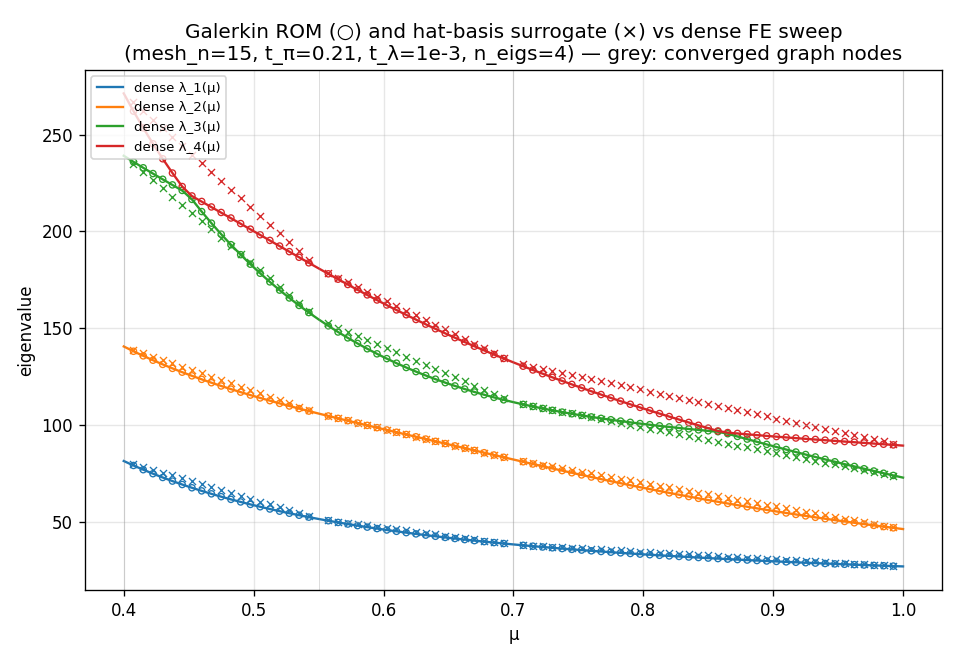
The four bands are tracked across the parameter range. The Galerkin ROM markers (○) sit tightly on the dense lines; the hat-basis crosses (×) follow the same curves but with visible piecewise-linear interpolation error between nodes. The crossing region is where the matching machinery earns its keep — both surrogates reproduce the correct band ordering there.
The accompanying regression checks assert the eigenvalue error ceilings for both surrogates; the plot here is the eyeball version.